DFS and BFS

Introduction

Depth-first search (DFS) and breadth-first search (BFS) are both algorithms used for traversing or searching graphs.

Depth-First Search

A DFS algorithm will start at an arbitrary node in a graph, and then explores as far as possible. When there are no more nodes left to explore, the algorithm backtracks to the previous node explored.

Example

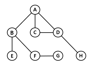
Lets do a depth-first search on the graph above starting at node A, assuming that nodes on the left are searched before the nodes on the right.

• First, we’ll go to node B, then E. Since there is nowhere else to go from E, we come back to B.
• Then, we’ll go to F to G, and come back to B because G is a dead end, and there is nowhere else to go from F.
• Now, we have been to all neighbouring nodes of B, so we come back to A, and move on to C.
• From C, we’ll move to D, and since we’ve already been to A, we’ll go to H.
• H is a dead end, there is nowhere to go from D and C, so we return back at A.
• There are no more nodes left unvisited that can be reached from A, thus we are done.

In conclusion, we traverse the nodes in the following order: A B E F G C D H

Similarly, if we started from B, the order of traversal woulde be: B E F G A C D H (assuming that nodes on the bottom are searched before nodes on the top)

Example Code

The following is an implementation of DFS in C++.

vector<int> traversal,graph[V+1];
bool visited[V+1];

void DFS(int u){
  visited[u] = true;
  traversal.push_back(u);
  for(int i = 0; i < graph[u].size(); i++){
    int next = graph[u][i];
    if(visited[next] == false)
      DFS(next);
  }
}

Variable explanation:

• graph: The adjacency list of the graph
• visited: A boolean array that keeps track of nodes that have been previously visited
• traversal: A vector that stores the nodes in the order they were traversed
• V: The number of nodes in the graph
• u: The node that is currently being searched
• next: The node that is going to be searched next

Simple code explanation:

First, node u is marked as visited using the visited array. Then node u is pushed into the traversal vector. Within the for loop, the if statement checks if each of the adjacent nodes of node u have been visited. If the next node hasn’t been visited, we continue searching from the next node using recursion.

The time complexity of the code above is $O(V+E)$.

Uses (DFS Spanning Tree)

There are many places where a DFS algorithm can be used. Here, I want to look at one use of the DFS algorithm; the DFS spanning tree.

A DFS spanning tree is a tree where the root node is the node where the DFS starts at. The shape of the tree can differ based on the order of traversal.

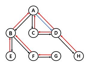
Each edge of a graph can be put into one of four groups: forward edges, back edges, cross edges, and tree edges. What group each edge belongs to is based on the spanning tree.

Here are the descriptions for each group:

• Tree edge: An edge that is part of the spanning tree. If a node V has been first visited using an edge (U, V), (U, V) is a tree edge.
• Back edge: An edge that points to from a node to one of its ancestors. Back edges have the property of being included within a cycle in the original graph.
• Forward edge: An edge that points from a node of a tree to one of its decendants that is not contained in the spanning tree.
• Cross edge: An edge which is neither of the above.

The following image shows the types of edge defined by the spanning tree of the graph we looked at before. Tree edges, back edges, and forward edges are represented using the colors black, red, and blue. As for cross edges, there exists none.

The following C++ code shows what type each edge is when inputed an edge list.

#include <iostream>
#include <vector>
using namespace std;

vector<int> graph[1000];
vector<int> discovered, finished;
int counter;

void DFS(int node)
{
  discovered[node] = counter++;

  for (int i = 0; i < graph[node].size(); ++i) {
    int next = graph[node][i];
    cout << "(" << node << "," << next << "): ";

    if (discovered[next] == -1) {
      cout << "tree edge" << endl;
      DFS(next);
    }
    else if (discovered[node] < discovered[next])
      cout << "forward edge" << endl;
    else if (finished[next] == 0)
      cout << "back edge" << endl;
    else
      cout << "cross edge" << endl;
  }
  finished[node] = 1;
}

int main(){
	int v,e,root;
	cin >> v >> e;
	discovered.resize(v+1);
	finished.resize(v+1);
	for(int i=0;i<e;i++){
		int a,b;
		cin >> a >> b;
		graph[a].push_back(b);
		//graph[b].push_back(a); //Uncommenting this line makes the inputed graph into a undirected graph
	}
	fill(discovered.begin(),discovered.end(),-1);
  cin >> root;
	DFS(root);
}

Variable explanation:

• graph: The adjacency list of the graph
• discovered: A vector that stores the order of when a node was visited, initialy set to -1
• finished: A vector that keeps track of whether a node has finished searching
• counter: The current order of the node visited
• v: The number of nodes in the graph
• e: The number of edges in the graph
• root: The node where the search starts

Simple code explanation:

Within the DFS function, if discovered[next] == -1, it means we never visited before, so the corresponding edge will be a tree edge. If discovered[next] is larger than discovered[node] it means that next is a decendant of node as it has been visited later, thus making the node a forward node. If discovered[next] is smaller, the edge will be a back edge if next is not finished searching, thus finished[next] == 0. Otherwise, the edge would be a cross edge.

Now that were done with depth-first search (which turned out longer than I expected), lets move on to breadth-first search.

Breadth-First Search

BFS is like DFS, but instead of going as deep as possible, it explores all of the nodes at the current depth, before moving on to the next depth level. In a BFS algorithm, a queue is usually required to keep track of child nodes that have been encountered, but not visited.

Example

Lets do a breadth-first search on the graph above, starting at node A, and assuming that nodes on the left are explored before nodes on the right.

• First, we will explore nodes B, C, and D as they are on the same depth. While exploring B, we encounter nodes E and F, and while exploring D, we encounter H.
• Those are the child nodes that are present in the next depth level, and thus we explore E, F, and H next. While exploring F, we encounter G, which again, is on the next depth level.
• Once we explore G, there are no more nodes left to explore, thus the searching ends.

In conclusion, we traverse the nodes in the following order: A B C D E F H G

Similarly, if we started at node B, the order of traversal would be: B E F A G C D H (assuming that nodes on the bottom are searched before nodes on the top)

Example Code

The following is an implementation of BFS in C++.

vector<int> traversal,graph[V+1];
bool visited[V+1];

void BFS(int node){
  queue<int> q;
  q.push(node);

  visited[node] = true;
  while(!q.empty()){
    int u = q.front();
    q.pop();
    traversal.push_back(u);
    
    for(int i = 0; i < graph[u].size(); i++){
      int v = graph[u][i];
      if(visited[v] == false){
        visited[v] = true;
        q.push(v);
      }
    }
  }
}

Variable explanation:

• graph: The adjacency list of the graph
• visited: A boolean array that keeps track of nodes that have been previously visited
• traversal: A vector that stores the nodes in the order they were traversed
• V: The number of nodes in the graph
• q: A queue to keep track of nodes that have been ecountered, but not searched
• u: The node that is currently searching
• v: The node on the next depth level that has been encountered

Simple code explanation:

The search begins by pushing the starting node into the queue and marking it as visited. Then, in the while loop, the front of the queue is put into the traversal vector, and then popped. The for loop searches all of the adjacent nodes of the popped node, and if it hasn’t been encountered yet, it puts it in the queue so it can be searched later. The process repeats untill the queue is empty, which means that there are no more nodes left to search.

Unlike DFS, a BFS implementation does not use recursion (DFS can also be implemented without recursion, but usually it’s easier to just use recursion).

The time complexity of the code above is $O(V+E)$.

Uses (Flood Fill Algorithm)

Just like DFS, there are many places where a BFS algorithm is used. Here, I want to look at one of those uses, namely the flood fill algorithm.

A flood fill algorithm finds and alters an area connected to a given node in a multi-dimensional array. It can be used in the ‘bucket’ fill tool of various paint programs, as well as games such as Minesweeper to determine which tiles should be cleared.

There are many ways to implement a flood fill algorithm, but here I’m going to show an implementation using BFS and a queue, in C++.

typedef pair<int,int> pii;

const int dr[] = {1, -1, 0, 0};
const int dc[] = {0, 0, 1, -1};

int R,C;
int grid[MAX][MAX];
bool visited[MAX][MAX];

void floodfill(int r, int c, int x){
  queue<pii> q;
  q.push({r,c});
  visited[r][c] = true;
  
  int col = grid[r][c];
  while(!q.empty()){
    pii cur = q.front();
    q.pop();
    grid[cur.first][cur.second] = x;
    for(int i = 0; i < 4; i++){
      int nr = cur.first + dr[i], nc = cur.second + dc[i];
      if(nr < 0 || nc < 0 || nr >= R || nc >= C) continue;
      if(visited[nr][nc] || grid[nr][nc] != col) continue;
      visited[nr][nc] = true;
      q.push({nr,nc});
    }
  }
}

Variable explanation:

• dr, dc: An array to make traversing a grid easier. When added together, each index represents south, north, east, west.
• R, C: The number of rows and column on the grid
• grid: A two-dimensional array that stores the grid
• visited: An array to keep track of whether a point has been visited while performing the algorithm
• MAX: The maximum number of rows and columns that can be inputed

Simple code explanation:

The code above functions exactly like the BFS code, with some minor differences. Since a grid is given rather than a graph, we can use the dr, dc arrays to traverse neighbouring points. Also, there are two if statements added to check wether the current point we are checking is inside the grid, and whether it has the same value as the initial point we started at. If not, the code ignores that point and continues. Other than that, it should be the same as the BFS code.

And with that, we are done.

Conclusion

I’m no expert, but I’m pretty sure DFS and BFS are important, so it would be a good idea to know how to implement them, and their uses. I only introduced one use for each, but there are lot more such as finding the number connected components, topology sort, checking whether a graph is bipartite, etc.